Category Archives: mcmc

Ergodicity of Combocontinuous Adaptive MCMC algorithms

February 15, 2017mcmc, Monte CarloIngmar

easy_adaptive_mcmc

This preprint by Jeff Rosenthal and Jinyoung Yang (currently available from Jeffs webpage) might also be called “Easily verifiable adaptive MCMC”. Jeff Rosenthal gave a tutorial on adaptive MCMC during MCMSki 2016 mentioning this work. Adaptive MCMC is based on the idea that one can use the information gathered from sampling a distribution using MCMC to improve the efficiency of the sampling process.

If two conditions, diminishing adaptation and containment are satisfied, an adaptive MCMC algorithm is valid in the sense of asymptotically consistent. Diminishing adaptation means that two consecutive Markov Kernels in the algorithm will be asymptotically equal. In other words, we either stop adaptation at some point or we know that the adaptation algorithm converges.
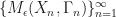
Containment means the number of repeated applications of all used Markov Kernels to get close to the target measure is bounded. Concretely, let $\gamma$ be a Markov kernel index, $P_\gamma^m(x,\cdot)$ be the distribution resulting from m-fold application of kernel $P_\gamma$ starting from $x$ . In other words start MCMC at point x with kernel $P_\gamma$ , let it run for m iterations and consider the induced distribution for the last point. Let $\pi$ be the target distribution. Then containment requires that
$\{M_\epsilon(X_n, \Gamma_n)\}_{n=1}^\infty$ is bounded in probability for all $\epsilon > 0$ . Here $M_\epsilon(x, \gamma) = \inf \{ m \geq 1 : \| P_\gamma^m(x,\cdot) - \pi(\cdot) \|_\textrm{TV}\}$ and $\|\cdot\|_\textrm{TV}\}$ is a worst case distance between distributions (total variation distance).

The paper is concerned with trying to find conditions for containment in adaptive MCMC that are more easily verified than those from earlier papers. First however it gives a kind of blueprint for adaptive algorithms that satisfy containment.

A blueprint for consistent adaptive MCMC

Nameley, let $\mathbb{R}^d$ be the support of the target distribution and $K \subseteq \mathbb{R}^d$ some large bounded region, $D > 0$ some large constant. The blueprint, Bounded Adaptive Metropolis, is the following:

Start the algorithm at some $X_0 \in K$ and fix a $d \times d$ covariance matrix $\Sigma_*$ . At iteration n generate a proposal $Y_{n+1}$ by

(1) $Y_{n+1} \sim \mathcal{N}(X_n, \Sigma_*)~\textrm{if}~X_n \notin K$
(2) $Y_{n+1} \sim \mathcal{N}(X_n, \Sigma_{n+1})~\textrm{if}~X_n \in K$

Reject if $|Y_{n+1} - X_{n}| > D$ , else accept with the usual Metropolis-Hastings acceptance probability. The $\Sigma_{n+1}$ can be chosen almost arbitrarily if the diminishing adaptation condition is met, so either the mechanism of choosing is fixed asymptotically or converges.

It would seem to me that we can actually change the distribution in (2) arbitrarily if we continue to meet diminishing adaptation. So for example we could use an independent metropolis, adaptive Langevin or other sophisticated proposal inside K, so long as condition (e) in the paper is satisfied, i.e. the adaptive proposal distribution used in (2) is continuous in $X_n$ . Which leads us to the actual conditions for containment.

General conditions for containment in adaptive MCMC

Let $\mathcal{X}$ be a general state space. For example in the Bounded Metropolis we had $\mathcal{X}=\mathbb{R}^d$ . The conditions the authors give are (even more simplified by me):

(a) The probability to move more than some finite distance D > 0 is zero: $Pr(|X_{n+1} - X_n| > D) = 0$
(b) Outside of K, the algorithm uses a fixed transition kernel P that never changes (and still respects that we can at most move D far away)
(c) The fixed kernel P is bounded above by $P(x, dy) \leq M \mu_*(dy)$ for finite constant M > 0 and all x that are outside K but no farther from it than D (call that set $K_D$ ) and all y that are between D and 2D distance from K (call that set $K_{2D} \backslash K_D$ ). Here $\mu_*$ is any distribution concentrated on $K_{2D} \backslash K_D$ .
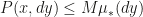
(d) The fixed kernel P is bounded below by $P^{n_0}(x, A) \geq \epsilon \nu_*(A)$ for some measure $\nu_*$ on $\mathcal{X}$ , some $n_0 \in \mathbb{N}$ and some event A.
(e) Let $\gamma$ be the parameter adapted by the algorithm. The overall proposal densities $q_\gamma(x,y)$ (combining the proposal in and outside of K) are continuous in $\gamma$ for fixed (x,y) and combocontinuous in x. Practically, this would be that the fixed proposal when outside K and the adaptive proposal when inside K are both continuous.

Here, conditions (a) and (b) are very easy to ensure even when not an expert on MCMC. Conditions (c) and (d) sound harder, but as mentioned above it seems to me that they are easy to ensure by just using a (truncated, i.e. respecting (a)) gaussian random walk proposal outside of K. Finally, (e) seems to boil down to making the adaptive proposal continuous in both $\gamma$ and x.

The proofs use a generalization of piecewise continuous functions and a generalized version of Dinis theorem to prove convergence in total variation distance.

This paper seems to me to be a long way from Roberts & Rosenthal (2007, Journal of Applied Probability) which was the first paper I read on ergodicity conditions for adaptive MCMC. It truly makes checking containment much easier. My one concern is that the exposition could be clearer for people that are not MCMC researchers. Then again, this is a contribution paper rather than a tutorial.

A Variational Analysis of Stochastic Gradient Algorithms

May 9, 2016big tall data, Inference, mcmc, Monte Carlo, stats, tall big data, Variational InferenceIngmar

This arXival by Mandt, Hoffman and Blei from February takes a look at what they call SGD with constant learning rate or constant SGD. Which is not really Stochastic Gradient Descent anymore, but rather a sampling algorithm, as we should bounce around the mode of the posterior rather than converging to it. Consequently they interpret constant SGD as a stochastic process in discrete time with some stationary distribution. They go on to analyse it under the assumption that the stationary distribution is Gaussian (Assumption 1 and 4). Something that springs to my mind here is the following: even if we accept that the stationary distribution of the process might be Gaussian (intuitively, not rigorously), what guarantees that the stationary distribution is the posterior? Even if the posterior is also gaussian, it could have a different (co)variance. I think a few more words about this question might be good. In particular, without adding artificial noise, is it guaranteed that every point in the posteriors domain can be reached with non-zero probability? And can be reached an infinite number of times if we collect infinite samples? If not, the constant SGD process is transient and does not enjoy good stability properties.

Another delicate point hides in Assumption 1: As our stochastic gradient is the sum of independent RVs, the CLT is invoked to assume that the gradient noise is Gaussian. But the CLT might not yet take effect if the number of data points in our subsample is small, which is the very thing one would like in order to have advantages in computation time. This of course is yet another instance of the dilemma common to all scalable sampling techniques, and at this stage of research this is not a show stopper.
Now assuming that constant SGD is not transient and it has a stationary distribution that is the posterior and that the posterior or its dominant mode is approximately Gaussian, we can of course try to optimize the parameters of constant SGD to make the sample it produces as close a possible to a posterior sample. Which the authors conveniently do using an Ornstein-Uhlenbeck approximation, which has a Gaussian stationary distribution. Their approach is to minimize KL-Divergence between the OU approximation and the posterior, and derive optimal parameter settings for constant SGD in closed form. The most interesting part of the theoretical results section probably is the one on optimal preconditioning in Stochastic Gradient Fisher Scoring, as that sampler adds artificial noise. Which might solve some of the transience questions.

The presentation would gain a lot by renaming “constant SGD” for what it is – a sampling algorithm. The terminology and notation in general are sometimes a bit confusing, but nothing a revision can’t fix. In general, the paper presents an interesting approach to deriving optimal parameters for a class of algorithms that is notoriously hard to tune. This is particularly relevant because the constant step size could improve mixing considerably over Welling & Tehs SGLD. What would be interesting to see is wether the results could be generalized to the case where the posterior is not Gaussian. For practical reasons, because stochastic VB/EP works quite well in the gaussian case. For theoretical reasons, because EP now even comes with some guarantees (haven’t read that paper admittedly). Maybe a path would be to take a look at the Gaussian approximation to a multimodal posterior spanning all modes, and minimizing KL-Divergence between that and the OU process. Or maybe one can proof that constant SGD (with artificial noise?) has some fixed stationary distribution to which stochastic drift term plus noise are a Markov Kernel, which might enable a pseudo-marginal correction.

Variational Hamiltonian Monte Carlo via Score Matching

April 26, 2016Inference, mcmc, Monte Carlo, Neural Networks, stats, Variational InferenceIngmar

This is an arXival (maybe by now ICML paper?) by Zhang, Shahbaba and Zhao. It suggest fitting an emulator/surrogate $q_\eta$ to the target density $\pi$ via score matching and then use the gradients of $q_\eta$ rather than those of $\pi$ for generating proposal with HMC. Their main selling point being that this decreases wall-clock time for HMC.

However, that seems to me like reselling the earlier paper by Heiko Strathmann and collaborators on Gradient-free Hamiltonian Monte Carlo with Efficient Kernel Exponential Families. Zhang et al use basically the same idea but fail to look at this earlier work. Their reasoning to use a neural network rather than a GP emulator (computation time) is a bit arbitrary. If you go for a less rich function class (neural network) then the computation time will go down of course – but you would get the same effect by using GPs with inducing points.

Very much lacking to my taste is reasoning for doing the tuning they do. Sometimes they tune HMC/Variational HMC to 85% acceptance, sometimes to 70% acceptance. Also, it seems they not adapting the mass matrix of HMC. If they would, I conjecture the relative efficiency of Standard HMC vs Variational HMC could change drastically. Details on how they tune SGLD is completely lacking.

Overall, I think it is not yet clear what can be learned from the work reported in the paper.

Marginal Likelihood From the Metropolis–Hastings Output

April 16, 2016mcmc, Models, Monte CarloIngmar

This is a rather old JASA paper by Siddhartha Chib and Ivan Jeliazkov from 2001. I dug it up again as I am frantically trying to get my contribution for the CRiSM workshop on Estimating Constants in shape. My poster will be titled Flyweight evidence estimates as it looks at methods for estimating model evidence (aka marginal likelihood, normalizing constant, free energy) that are computationally very cheap when a sample from the target/posterior distribution exists.
I noticed again that the approach by Chib & Jeliazkov (2001) does not satisfy this constraint, although they claim otherwise in the paper. The estimator is based on the fact that the normalized probability of a point $\theta^*$ under the target when using Metropolis Hastings is

where $q$ is the proposal density, $\alpha$ the acceptance probability and $y$ the data. If $\bar\pi$ is the unnormalized target, we can get the evidence estimate $Z = \bar\pi (\theta^*|y)/\pi(\theta^*|y)$ .
Now the integral in the numerator is cheap to estimate when we already have samples from $\pi$ . The authors claim that because it is cheap to sample from $q$ , the denominator is cheap as well. I can’t help it: this statement feels a bit deceptive to me. While indeed samples from $q$ are cheep to generate, evaluating $\alpha(\theta^*,\theta^{(j)}|y)$ for each sample $\theta^{(j)} \sim q(\theta^*,\cdot|y)$ is the opposite of cheap! It involves evaluating $\bar\pi(\theta^{(j)}|y)$ for all j, which is basically the same cost as getting samples from the target in the first place.
I already included that criticism in my PhD thesis, but when revising under time pressure I no longer thought it was valid and erroneously took it out.

Non-asymptotic convergence analysis for the Unadjusted Langevin Algorithm

April 15, 2016Inference, mcmc, Monte Carlo, Numerics, statsIngmar

This is an important arXival by Alain Durmus and Eric Moulines. The title is slightly optimized for effect, as the paper actually contains non-asymptotic and asymptotic analysis.

The basic theme of the paper is in getting upper bounds on total variation (and more general distribution distances) between an uncorrected discretized Langevin diffusion wrt some target $\pi$ and $\pi$ itself. The discretization used is the common scheme with the scary name Euler-Maruyama:

$X_{k} \sim \mathcal{N}(\cdot|X_{k-1} + \gamma_{k}\nabla \log \pi(X_{k-1}), \sqrt{2\gamma_{k}I} = R_{\gamma_{k}}(\cdot |X_{k-1})$

Under a Foster-Lyapunov condition, $R_{\gamma_{k}}$ is a Markov kernel that admits a unique stationary distribution $\pi_{\gamma_{k}}$ that is close to the desired $\pi$ in total variation distance and gets closer when $\gamma_{k}$ decreases.

Now in the non-asymptotic case with fixed $\gamma = \gamma_k$ , the authors provide bounds that explicitly depend on dimensionality of the support of the target, the number of samples drawn and the chosen step size $\gamma$ . Unfortunately, these bounds contain some unknowns as well, such as the Lipschitz constant $L$ of the gradient of the logpdf $\log \pi(\cdot)$ and some suprema that I am unsure how to get explicitly.

Durmus and Moulines particularly take a look at scaling with dimension under increasingly strong conditions on $\pi$ , getting exponential (in dimension) constants for the convergence when $\pi$ is superexponential outside a ball. Better convergence can be achieved when assuming $\pi$ to be log-concave or strongly log-concave. This is not surprising, nevertheless the theoretical importance of the results is clear from the fact that together with Arnak Dalalyan this is the first time that results are given for the ULA after the Roberts & Tweedie papers from 1996.

As a practitioner, I would have wished for very explicit guidance in picking $\gamma$ or the series $\{\gamma_k\}_{k=1}^\infty$ . But hopefully with Alains paper as a foundation that can be the next step. As a non-mathematician, I had some problems in following the paper and at some point I completely lost it. This surely is in part due to the quite involved content. However, one might still manage to give intuition even in this case, as Sam Livingstones recent paper on HMC shows. I hope Alain goes over it again with readability and presentation in mind so that it will get the attention it deserves. Yet another task for something that already took a lot of work…

(photo: the Lipschitz Grill diner in Berlin – I don’t
know about their food, but the name is remarkable)

On the Geometric Ergodicity of Hamiltonian Monte Carlo

February 10, 2016Inference, mcmc, Monte Carlo, Numerics, statsIngmar

This remarkable arXival by Sam Livingstone, Betancourt, Byrne and Girolami takes a look at the conditions under which Hybrid/Hamiltonian Monte Carlo is ergodic wrt a certain distribution $\pi$ , and, in a second step, under which it will converge in total variation at a geometric rate. A nice feature being that they even prove that setting the integration time dynamically can lead to the sampler yielding geometric rate for a larger class of targets. Under idealized conditions for the dynamic integration time and, admittedly, in a certain exponential family.

Whats great about this paper, apart from the results, is how it manages to give the arguments in a rather accessible manner. Considering the depth of the results that is. The ideas are that

the gradient should at most grow linearly
for the gradient of $\pi$ to be of any help, it cannot lead further into the tails of the distribution or vanish (both assumption 4.4.1)
as we approach infinity, every proposed point thats closer to the origin will be accepted (assumption 4.4.2)

If the gradient grows faster than linear, numerics will punch you in the face. That happened to Heiko Strathmann and me just 5 days ago in a GradientIS-type algorithm, where an estimated gradient had length $10^{144}$ and led to Nirvana. If not the estimation is the problem but the actual gradient, of course you have the same effect. The second assumption is also very intuitive: if the gradient leads into the tails, then it hurts rather than helps convergence. And your posterior is improper. The final assumption basically requires that your chance to improve by proposing a point closer to the origin goes to $1$ the further you move away from it.

A helpful guidance they provide is the following. For a class of exponential family distributions given by $exp(-\alpha|x|^\beta)~\forall \alpha,\beta >0$ , whenever the tails of the distribution are no heavier than Laplace ( $\beta \geq 1$ ) and no thinner than Gaussian ( $\beta \leq 2$ ), HMC will be geometrically ergodic. In all other cases, it won’t.

Another thing that caught my eye was their closed form expression for the proposal after $L$ leapfrog steps with stepsize $\epsilon$ , eq. (13):

Capture d’écran 2016-02-09 à 21.28.00

Which gives me hope that one should be able to compute the proposal probability after any number of leapfrog steps as long as $\nabla \log \pi$ is invertible and thus a Jacobian exists to account for the transformation of $p_0$ hidden in the $x_{i\epsilon}$ . A quick check with $\pi$ given by a bayesian posterior shows that this might not be trivial however.

A comparison of generalized hybrid Monte Carlo methods with and without momentum flip

February 8, 2016Importance Sampling, mcmc, Monte CarloIngmar

This experimental paper from 2009 by Akhmatskaya, Bou-Rabee and Reich in the Journal of Computational Physics takes a look at what in statistics people would call HMC with partial momentum refreshment.The paper got my attention mainly because I met Elena Akhmatskaya at MCMSki.

The ‘generalized’ in the paper refers to the fact that the momenta are not resampled at each new HMC step, but rather according towhere $p_i \sim \mathcal{N}(0,\Sigma)$ is the old momentum, and we mix it with another Gaussian RV of the same distribution $u_i$ for some parameter $\phi$ . We recover HMC for $\phi=\pi/2$ , as in that case the momentum is always refreshed.

Also, they are looking at a so-called shadow HMC variant, which really samples from a Hamiltonian system that is not the original one, but close to it. Correction for sampling from the wrong distribution is done by importance weighting (when she was telling me that I thought “I knew IS could work in high dimensions!”, as they sample from up to 10,000 dimensions and do better than HMC!).

Now the main gist of the paper is that they where trying to get rid of momentum flips in the case of rejection of the proposal, as it was previously thought that momentum flips lead to a worse sampler. The intuition would be that a momentum flip leads you back to where you started. However, the finding is that to the contrary, their version without flip (that still satisfies a detailed balance criterion) does worse in actual estimation tasks than the conservative Generalized Shadow HMC (GSHMC) sampler. I like when things stay easy. But as this paper does not describe the actual GSHMC method in detail, I will have to go back to the original paper, as my interest is sparked.

A Repulsive-Attractive Metropolis Algorithm for Multimodality

January 26, 2016Inference, mcmc, Monte CarloIngmar

(Title image from Wikipedia)

Christian put my nose on this preprint by Tak, Meng and van Dyk a few days ago, so during the flight from Berlin to Paris today I sniffed on it. It was a very interesting read and good to get my thoughts away from the fact that I was an Opfer of German friendliness at airport security.
The basic idea is to design a random walk MH algorithm for targets with multiple and distant modes. The distant is important here, because for very close modes simple Adaptive Metropolis (Haario et al. 2001), which is simply using a scaled version of the targets covariance in a Gaussian random walk, should work pretty well.

Which it probably does not for the targets above, as such a proposal would often end up in areas of low posterior density.
Now the idea is the following: given current state $x_i$ of the Markov Chain, the final MH proposal $x''$ is constructed using an intermediate step $x'$ , where the intermediate step is encouraged to have lower density than $x_i$ under the target, while $x''$ is encouraged to have higher density than the intermediate step. Hoping that the intermediate step gets you out of a mode and the consecutive step into a new mode. This is achieved by using the inverse MH-ratio for encouraging moves to a valley in the target, while the standard MH-ratio is used for moving uphill again. Of course computing the final acceptance probability $\alpha(x''|x_i)$ involves computing an intractable integral, as one has to integrate away the intermediate downhill move. They get around this by introducing an auxiliary variable, a technique inspired by Møller et al. (2006), where it was used to get around the computation of normalizing constants. I discussed a similar idea shortly with Jeff Miller (currently at Duke) one and a half years ago when we worked on the estimation of normalizing constants though using gradient information.
Am main argument for their algorithm is that it only needs tuning of a single scale parameter, whereas other MCMC techniques for multimodal targets are notoriously hard to tune.
In evaluation they compare to tempered transitions and equi-energy samplers and perform better both with respect to computing time and MSE. And of course human time invested in tuning.
However, I’m slightly tempted to repeat Nicolas mantra here “just use SMC”. Or slightly change the mantra to “… PMC” – because this is easier to stomach for MCMC-biased researchers, or so I believe. Of course this adds the number of particles to tuning, but that might be tuned automatically using the recent paper of the Spanish IS-connection.

Layered adaptive Importance Sampling

January 25, 2016Inference, mcmc, SMCIngmar

This arXival from last spring/summer by Martino, Elvira, Luengo and Corander combines and extends upon recent advances of Importance Sampling, using mainly ideas from Adaptive Multiple lmportance Sampling (AMIS) and Population Monte Carlo (PMC). The extension consists of the idea to not use the Importance Sampling procedure itself to come up with new proposal distributions, but rather to run a Markov Chain. The output of which is used solely as the location parameter for IS proposal distributions $q_{n,t}$ . The weights of the samples drawn from these are Rao-Blackwellized using the deterministic mixture idea of Zhou and Owen, and as far as I can see only the Importance Samples are used for estimating integrands.
What’s most striking for me as somebody who has thought about these methods a lot during the PhD is the idea that in principle one is free to Rao-Blackwellize using an arbitrary partition of the samples/proposal distributions and still get a consistent estimator. Xi’an mentioned this to me earlier and of course it is not surprising given that even without Rao-Blackwell my Gradient IS did considerably better than some Adaptive MCMC algorithms. However this paper makes that idea transparent and uses it extensively. The main idea that is put forward however is to use (parallel) MCMC with the same target for coming up with IS-proposal locations. The output of MCMC is only used for that purpose but not for estimation. Which seems kind of wasteful, but in a nice conversation over email the first author Luca Martino assured me that recycling proposals as both IS and MH proposals made performance go down because of correlations. I don’t get an intuition for why that would be the case, but maybe I’ll have to fall on my own nose for that. What I like about this particular idea of getting locations from MCMC is that one is free from the tuning problem I’ve hit upon in GRIS: if you scale up the proposal covariance in GRIS (or in the PMC approach from the Cappé 2004 paper), you can get an arbitrarily high ESJD – together with a really bad target approximation. Thus unmodified ESJD cannot be used for tuning. And neither can acceptance rate which doesn’t exist. Using MCMC for getting proposal locations is an elegant way around that problem. The effect of this is shown in the plot from the paper below, where the two rightmost plots show one of their methods.

Some other aspects about the paper I find less clear. For instance, I’m not sure about the abundance of different algorithms that are introduced. It leaves the impression that the authors where trying to do mass instead of class (something I might make myself guilty of these weeks as well). Also, while the targets they use for evaluation are fine, only reporting the MSE of one dimension of one integrand seems odd. One simple thing here might be to report the MSE averaged over dimensions as well, another to report the MSE of an estimate of the target distributions variance/higher order moments.

(Title image (c) Carlos Delgado, CC-BY-SA)

Why the MAP is a bad starting point in high dimensions

January 21, 2016Inference, mcmc, Monte Carlo, SMC, statsIngmar

During MCMSki 2016, Heiko mentioned that in high dimensions, the MAP is not a particularly good starting point for a Monte Carlo sampler, because there is no volume around it. I and several people smarter than me where not sure why that could be the case, so Heiko gave us a proof by simulation: he sampled from multivariate standard normals with increasing dimensions and plotted the euclidean norm of the samples. The following is what I reproduced for sampling a standard normal in $D=30$ dimensions.The histogram has a peak at about $\sqrt{D}$ , which means most of the samples are in a sphere around the mean/mode/MAP of the target distribution and none are at the MAP, which would correspond to norm $0$ .

We where dumbstruck by this, but nobody (not even Heiko) had an explanation for what was happening. Yesterday I asked Nicolas about this and he gave the most intuitive interpretation: Given a standard normal variable in $D$ dimensions, $x \sim \mathcal{N}(0,I_D)$ , computing the euclidean norm you get $n^2 = \|x\|^2 = \sum_{i=1}^D x_i^2$ . But as $x$ is gaussian, this just means $n^2$ has a $\chi^2(D)$ distribution, which results in the expected value $\mathbb{E}(n) = \sqrt{D}$ . Voici l’explication.

(Title image (c) Niki Odolphie)