This preprint by Jeff Rosenthal and Jinyoung Yang (currently available from Jeffs webpage) might also be called “Easily verifiable adaptive MCMC”. Jeff Rosenthal gave a tutorial on adaptive MCMC during MCMSki 2016 mentioning this work. Adaptive MCMC is based on the idea that one can use the information gathered from sampling a distribution using MCMC to improve the efficiency of the sampling process.
If two conditions, diminishing adaptation and containment are satisfied, an adaptive MCMC algorithm is valid in the sense of asymptotically consistent. Diminishing adaptation means that two consecutive Markov Kernels in the algorithm will be asymptotically equal. In other words, we either stop adaptation at some point or we know that the adaptation algorithm converges.
Containment means the number of repeated applications of all used Markov Kernels to get close to the target measure is bounded. Concretely, let  be a Markov kernel index,
  be the distribution resulting from m-fold application of kernel
  starting from
  . In other words start MCMC at point x with kernel , let it run for m iterations and consider the induced distribution for the last point. Let
  be the target distribution. Then containment requires that
 is bounded in probability for all
  . Here
  and
and  is a worst case distance between distributions (total variation distance).
The paper is concerned with trying to find conditions for containment in adaptive MCMC that are more easily verified than those from earlier papers. First however it gives a kind of blueprint for adaptive algorithms that satisfy containment.
A blueprint for consistent adaptive MCMC
Nameley, let  be the support of the target distribution and
  some large bounded region,
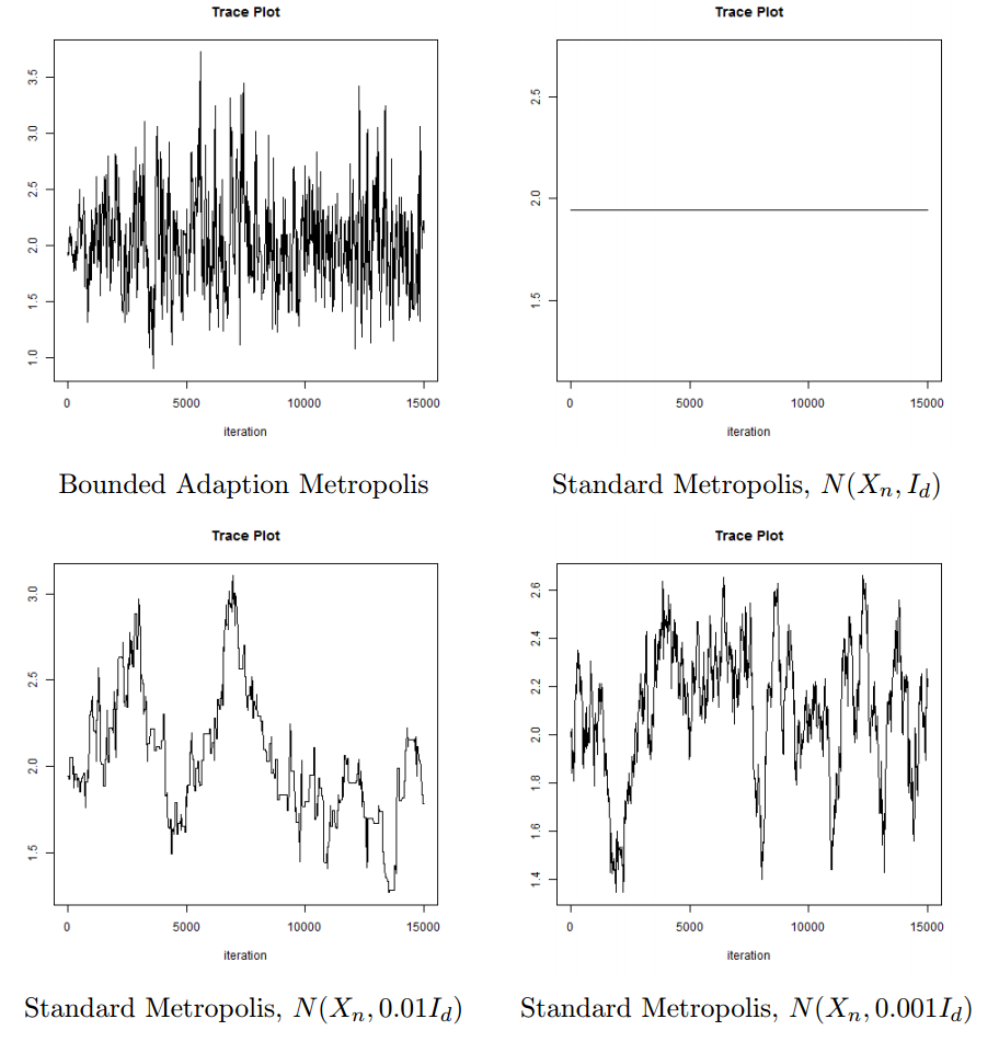
  some large constant. The blueprint, Bounded Adaptive Metropolis, is the following:
Start the algorithm at some  and fix a
  covariance matrix
  . At iteration n generate a proposal
  by
by
(1)
(2)
Reject if  , else accept with the usual Metropolis-Hastings acceptance probability. The
  can be chosen almost arbitrarily if the diminishing adaptation condition is met, so either the mechanism of choosing is fixed asymptotically or converges.
It would seem to me that we can actually change the distribution in (2) arbitrarily if we continue to meet diminishing adaptation. So for example we could use an independent metropolis, adaptive Langevin or other sophisticated proposal inside K, so long as condition (e) in the paper is satisfied, i.e. the adaptive proposal distribution used in (2) is continuous in  . Which leads us to the actual conditions for containment.
General conditions for containment in adaptive MCMC
Let  be a general state space. For example in the Bounded Metropolis we had
  . The conditions the authors give are (even more simplified by me):
(a) The probability to move more than some finite distance D > 0 is zero: 
(b) Outside of K, the algorithm uses a fixed transition kernel P that never changes (and still respects that we can at most move D far away)
(c) The fixed kernel P is bounded above by 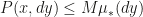 for finite constant M > 0 and all x that are outside K but no farther from it than D (call that set
  ) and all y that are between D and 2D distance from K (call that set
  ). Here
  is any distribution concentrated on .
(d) The fixed kernel P is bounded below by  for some measure
  on , some
  and some event A.
(e) Let be the parameter adapted by the algorithm. The overall proposal densities  (combining the proposal in and outside of K) are continuous in for fixed (x,y) and combocontinuous in x. Practically, this would be that the fixed proposal when outside K and the adaptive proposal when inside K are both continuous.
Here, conditions (a) and (b) are very easy to ensure even when not an expert on MCMC. Conditions (c) and (d) sound harder, but as mentioned above it seems to me that they are easy to ensure by just using a (truncated, i.e. respecting (a)) gaussian random walk proposal outside of K. Finally, (e) seems to boil down to making the adaptive proposal continuous in both and x.
The proofs use a generalization of piecewise continuous functions and a generalized version of Dinis theorem to prove convergence in total variation distance.
This paper seems to me to be a long way from Roberts & Rosenthal (2007, Journal of Applied Probability) which was the first paper I read on ergodicity conditions for adaptive MCMC. It truly makes checking containment much easier. My one concern is that the exposition could be clearer for people that are not MCMC researchers. Then again, this is a contribution paper rather than a tutorial.


 denote samples from the prior with density
  (the
(the  that follow the posterior density
  (the
(the  meaning analyzed), preferably without introducing unequal weights. Let the likelihood term be denoted by
  where
where  is the data and let
  be the normalized importance weight. The normalization in the denominator stems from the fact that in Bayesian inference we can often only evaluate an unnormalized version of the posterior
  .
. , while
  . Now we construct a joint probability between the discrete random variables distributed according to
  and those distributed according to
  , i.e. a matrix
  with non-negative entries summing to 1 which has the column sum
  be the joint pmf induced by
  under the additional constraint of cyclical monotonicity. This boils down to a linear programming problem. For a fixed prior sample
  this induces a conditional distribution over the discretely approximated posterior given the discretely approximated prior
  .
. . Instead, the paper proposes a deterministic transformation using the expected value
  . Reich proves that the mapping
  induced by this transformation is such that for
  ,
,  for
for  . In other words, if the ensemble size M goes to infinity, we indeed get samples from the posterior.
 Of course, this is not a problem when M is infinite, but my intuition would be that it has a rather strong effect in our finite world. One remedy here would of course be to introduce a rejuvenation step as in SMC, for example moving each particle
  using MCMC steps that leave
  invariant.
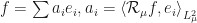
 . It’s called Operator VI as a fancy way to say that one is flexible in constructing how exactly the objective function uses
  and test functions from some family
  . I completely agree with the motivation: KL-Divergence in the form
  indeed underestimates the variance of $\pi$ and approximates only one mode. Using KL the other way around,
  takes all modes into account, but still tends to underestimate variance.
 to a bimodal distribution. However their method is not the only one to get bimodality by transforming a standard normal variable and actually the Jacobian correction can be computed even for their suggested transformation! The problem they encounter really is that they throw away one dimension of
  , which makes the tranformation lose injectivity. However by not throwing the variable away, we keep injectivity and it is possible to compute the density of the transformed variables. The reasons for not accessing the density

 be the loss for the parameter at
  and jth data point, then the usual batch gradient descent update is
  with
with  as step size.
 and uses the update
  , usually with a decreasing step size
  , observe that
  has an expected value of 0 and is thus a possible control variate. With the possible downside that whenever
  for the individual data points and then shows that the proposed procedure (termed stochastic variance reduced gradient or SVRG) enjoys geometric convergence. Even though the proof uses a slightly odd version of the algorithm, namely where
  . Rather simply setting
  should intuitively improve convergence, but the authors could not report a result on that. Overall a very nice idea, and one that has been discussed in more papers quite a bit, among others by Simon Lacoste-Julien and Francis Bach.