Category Archives: big tall data

Accelerating Stochastic Gradient Descent using Predictive Variance Reduction

During the super nice International Conference on Monte Carlo techniques in the beginning of July in Paris at Université Descartes (photo), which featured many outstanding talks, one by Tong Zhang particularly caught my interest. He talked about several variants of Stochastic Gradient Descent (SGD) that basically use variance reduction techniques from Monte Carlo algorithms in order to improve the convergence rate versus vanilla SGD. Even though some of the papers mentioned in the talk do not always point out the connection to Monte Carlo variance reduction techniques.

One of the first works in this line, Accelerating Stochastic Gradient Descent using Predictive Variance Reduction by Johnson and Zhang, suggests using control variates to lower the variance of the loss estimate. Let L_j(\theta_{t-1}) be the loss for the parameter at t-1 and jth data point, then the usual batch gradient descent update is \theta_{t} =\theta_{t-1} - \frac{\eta_t}{N} \sum_{j=1}^N\nabla L_j(\theta_{t-1}) with \eta_t as step size.

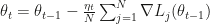
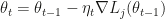
In naive SGD instead one picks a data point index uniformly j \sim \mathrm{Unif}(\{1,\dots,N\}) and uses the update \theta_{t} =\theta_{t-1} - \eta_t \nabla L_j(\theta_{t-1}), usually with a decreasing step size \eta_t to guarantee convergence. The expected update resulting from this Monte Carlo estimate of the batch loss is exactly the batch procedure update. However the variance of the estimate is very high, resulting in slow convergence of SGD after the first steps (even in minibatch variants).

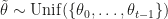
The authors choose a well-known solution to this, namely the introduction of a control variate. Keeping a version of the parameter that is close to the optimum, say \tilde\theta, observe that \nabla L_j(\tilde\theta) -  \frac{1}{N} \sum_{i=1}^N  \nabla L_i(\tilde\theta) has an expected value of 0 and is thus a possible control variate. With the possible downside that whenever \tilde\theta is updated, one has to go over the complete dataset.

The contribution, apart from the novel combination of knowledge, is the proof that this improves convergence. This proof assumes smoothness and strong convexity of the overall loss function and convexity of the L_j for the individual data points and then shows that the proposed procedure (termed stochastic variance reduced gradient or SVRG) enjoys geometric convergence. Even though the proof uses a slightly odd version of the algorithm, namely where \tilde\theta \sim\mathrm{Unif}(\{\theta_0,\dots,\theta_{t-1}\}). Rather simply setting  \tilde\theta = \theta_{t-1} should intuitively improve convergence, but the authors could not report a result on that. Overall a very nice idea, and one that has been discussed in more papers quite a bit, among others by Simon Lacoste-Julien and Francis Bach.

Exponential growth as plotted by my son


IMG_20160619_134418072With my son, my niece, sister and her boyfriend I visited the science museum in Mannheim about two months ago. There where many nice experiments, and as a (former ?) computer scientist I was particularly impressed by Leibniz’ mechanical digital calculator, completed in the 17th century and able to do all four basic arithmetic operations. This of course is another example for the superiority of Leibniz over Newton
One piece was a pure exhibit with no experiments: a system of cogwheels connected sequentially, where each added wheel took ten times longer for one complete cycle compared to the one before. While the first wheel needed five seconds, the 17th and last one did not seem to move, and indeed it completes a cycle about every 1.6 billion years (5*10^{16}\mathrm{sec}).
This is an example of exponential growth of course, so I told him the rice on chessboard story, e.g. the idea that starting with one grain of rice on the first square of a chessboard and doubling it on the next leads to loads and loads of rice. When he asked for rice this weekend I was rather unsuspecting, until he spilled some of it and asked for our help cleaning it up. He started the first four squares (though with linear growth as he didn’t remember completely) and we completed the first row together – after which I started simply weighing the rice, as counting took about a second per grain and already for the 256 grains on h2 I was too impatient, let alone  the 1024 for f2, which would have taken about 16 minutes to count. If this little exercise doesn’t drive home what exponential growth means, I don’t know what would.

A Variational Analysis of Stochastic Gradient Algorithms

This arXival by Mandt, Hoffman and Blei from February takes a look at what they call SGD with constant learning rate or constant SGD. Which is not really Stochastic Gradient Descent anymore, but rather a sampling algorithm, as we should bounce  around the mode of the posterior rather than converging to it. Consequently they interpret constant SGD as a stochastic process in discrete time with some stationary distribution. They go on to analyse it under the assumption that the stationary distribution is Gaussian (Assumption 1 and 4). Something that springs to my mind here is the following: even if we accept that the stationary distribution of the process might be Gaussian (intuitively, not rigorously), what guarantees that the stationary distribution is the posterior? Even if the posterior is also gaussian, it could have a different (co)variance. I think a few more words about this question might be good. In particular, without adding artificial noise, is it guaranteed that every point in the posteriors domain can be reached with non-zero probability? And can be reached an infinite number of times if we collect infinite samples? If not, the constant SGD process is transient and does not enjoy good stability properties.

Another delicate point hides in Assumption 1: As our stochastic gradient is the sum of independent RVs, the CLT is invoked to assume that the gradient noise is Gaussian. But the CLT might not yet take effect if the number of data points in our subsample is small, which is the very thing one would like in order to have advantages in computation time. This of course is yet another instance of the dilemma common to all scalable sampling techniques, and at this stage of research this is not a show stopper.
Now assuming that constant SGD is not transient and it has a stationary distribution that is the posterior and that the posterior or its dominant mode is approximately Gaussian, we can of course try to optimize the parameters of constant SGD to make the sample it produces as close a possible to a posterior sample. Which the authors conveniently do using an Ornstein-Uhlenbeck approximation, which has a Gaussian stationary distribution. Their approach is to minimize KL-Divergence between the OU approximation and the posterior, and derive optimal parameter settings for constant SGD in closed form. The most interesting part of the theoretical results section probably is the one on optimal preconditioning in Stochastic Gradient Fisher Scoring, as that sampler adds artificial noise. Which might solve some of the transience questions.

The presentation would gain a lot by renaming “constant SGD” for what it is – a sampling algorithm. The terminology and notation in general are sometimes a bit confusing, but nothing a revision can’t fix. In general, the paper presents an interesting approach to deriving optimal parameters for a class of algorithms that is notoriously hard to tune. This is particularly relevant because the constant step size could improve mixing considerably over Welling & Tehs SGLD. What would be interesting to see is wether the results could be generalized to the case where the posterior is not Gaussian. For practical reasons, because stochastic VB/EP works quite well in the gaussian case. For theoretical reasons, because EP now even comes with some guarantees (haven’t read that paper admittedly). Maybe a path would be to take a look at the Gaussian approximation to a multimodal posterior spanning all modes, and minimizing KL-Divergence between that and the OU process. Or maybe one can proof that constant SGD (with artificial noise?) has some fixed stationary distribution to which stochastic drift term plus noise are a Markov Kernel, which might enable a pseudo-marginal correction.

On Markov Chain Monte Carlo methods for tall data

The preprint by Rémi Bardenet, Arnaud Doucet and Chris Homes offers a very well written overview and some original contributions regarding MCMC with large datasets (I like ‘tall’ – maybe high dimensional posteriors could then be ‘fat’ and problems which exhibit both are the worn-out ‘big’ ?-).

Their original contributions revolve around using ideas from Firefly MC (developed by the authors of the Stochastic Optimization is Variational inference paper) on bounds for the likelihood with their Confidence sampler. I must say I wasn’t able to follow in detail and will have to read up on Firefly and the original Confidence sampler paper. One downside I see is that targets need to be differentiable (thrice for their bounds using Taylor approximations) and thus in particular continuous. While in general I try to avoid discrete models simply because you cant use gradient information, sometimes they are necessary. And better make progress on something slightly limited than not make progress.

In their review section, they clearly advise against divide-and-conquer approaches for tall data, i.e. approaches that sample from posteriors involving only part of the data and than combining the information somehow. The main reason for this being that the currently existing upper bounds suggest that the MSE of divide-and-conquer approaches could grow exponential in the number of batches. Thus one would have to use few, large batches, defeating the whole purpose of special methods for tall data.

The section finally exposed me to the delayed acceptance approach of Marco Banterle et al. which I meant to read for quite some time (and will read in the original). I found this approach to be very appealing for its elementary formulation. Most other approaches, including Bardenet, Doucet and Homes, are quite involved. I have to look into the objection regarding ergodicity of delayed acceptance raised by Bardenet, which could potentially be quite a problem of course.

A word about the evaluation section: I think its unfortunate that two of four experiments use logistic regression. The logistic regression target is very close to Gaussian, where MCMC is usually slammed by a simple EP approach (Leave Pima Indians alone!). And EP is easy to apply in the big data setting, or thats what I’ve heard. About the gamma regression target I don’t know, might be that EP does not do so well in that case.