Category Archives: stats

Supervised learning with quantum enhanced feature spaces

June 14, 2019Inference, RKHS, Variational InferenceIngmar

This letter to Nature (also on arXiv) by Havlicek and coauthors deals with gaining a quantum computing advantage for classification problems and is written by quantum physicists. The main reason a friend brought this to my attention is that the classification problem is solved using support vector machines, thus fitting my recent interest in reproducing kernel Hilbert space (RKHS) methods.
The main idea is that the way numerical data is encoded into a quantum state can result in a nonlinear feature map into the very high dimensional quantum Hilbert space. Consecutive computation in the quantum Hilbert space then induces nonlinear methods in the input space. In this case nonlinear classification.

The main contributions over papers that are easier to read coming from an RKHS background (such as Quantum machine learning in feature Hilbert spaces by Schuld et al) are twofold. For one, Havlicek and coauthors use a feature map that does not result in a trivial/useless RKHS. Specifically they propose to use two layers of a diagonal gate and a Hadamard gate and conjecture that this gives a quantum advantage (while a single layer can be simulated classically). I am quite lost here of course without any background in quantum computing. Second, their classification algorithm was implemented and run on an actual quantum computer, rather than simulated on standard computers. In particular, they use five superconducting transmons, which seems to be a type of qubit implementation and allows for quantum coupling.

The classification problem they tackle is a toy problem that they construct so as to be perfectly separable with their classification algorithm, which is of course a good sanity check for this first step of developing actual quantum machine learning. The decision of the algorithm for any of the two classes however cannot be read from the computing device deterministically, but only stochastically. The solution, seemingly common in quantum computing, is to read out the class repeatedly to obtain samples and compute their empirical average.
The training then consists of optimizing a bias variable and a parameter $\theta$ that determines the feature map (unless I’m mistaken!) so as to minimize the empirical missclassification error for the training dataset $R_{\mathrm{emp}}(\vec{\theta})=\frac{1}{|T|} \sum_{\vec{x} \in T} \mathrm{Pr}(\tilde{m}(\vec{x}) \neq m(\vec{x}))$ , where $\tilde{m}(\vec{x})$ is the label assigned by the algorithm and $m(\vec{x})$ is the actual label of $\vec{x}$ .

They use two main approaches, one working directly in the space spanned by the $\phi(\vec{x})$ at input points and finding a separating hyperplane in the quantum hilbert space directly. This is what they call the variational algorithm. The other approach uses the canonical Aronszajn features, i.e. the mapping of an input point $\vec{x}$ to the function $\langle\phi(\vec{x}), \cdot\rangle$ , and then construct a separating hyperplane as a linear combination of the functions induced by the training points.

Personally, I would think that the variational approach makes much more sense in the mid to long term, as the canonical approach does not yield a more powerful method but induces large memory cost for large datasets. Then on the other hand I’m completely lost when thinking about how to invert a matrix in the quantum feature space or compute solutions of systems of linear equations.

Overall, I think that this is a very interesting path to follow and am keen on finding out how quantum computing and machine learning/statistics might combine in beneficial ways.

Kernel conditional density operators

May 31, 2019Inference, RKHSIngmar

We recently submitted and arXived our new work on (conditional) density reconstruction methods using the reproducing kernel Hilbert space (RKHS) formalism. This is work with relentless PhD candidate Mattes Mollenhauer, Stefan Klus and Krikamol Muandet. It seeks to provide theory for an idea that came up over the course of working on eigendecompositions of RKHS operators and was catalysed by a characterization of the kernel mean embedding (KME) object, aka the classical kernel density estimate (KDE)/Parzen window estimate, that Stefan derived in another paper.

The key insight that we started out with is the follwing. Let $\mu_\mathbb{P} = \int k(x,\cdot) \mathrm{d}\mathbb{P}(x)$ be the KME/KDE functional for a density $p$ (with respect to reference measure $\rho$ ) of distribution $\mathbb{P}$ , and assume that this density is in the RKHS. Then $\mu_\mathbb{P} = C_\rho p$ , where $C_\rho$ is the covariance operator with respect to the reference measure. Thus we can recover $p$ by solving the inverse problem, i.e. in terms of the pseudo inverse $p = C^\dagger_\rho \mu_\mathbb{P}$ .
This is stated in Fukumizus Kernel Bayes rule paper for the general case of Radon-Nikodym derivatives, and later on in our work, though we didn’t realize the connections at first. So to be more precise: if the reference measure is Lebesgue, we estimate densities in the usual sense. In general Radon-Nikodym derivatives are estimated, i.e. $p = \mathrm{d}\mathbb{P}/\mathrm{d}\rho$ .

*Estimated density (green) starting from kernel mean embedding (red).*
*Ground truth in black.*

A first impression of the resulting estimates is given above. When choosing Lebesgue measure as the reference, we can estimate the density in the usual sense as given by the green curve using 200 samples from the true black density. Using a Tikhonov approach, we prove dimensionality-independent bounds on the stochastic error of this reconstruction depending mostly on the norm of the KME/KDE function and the number of samples.

The real power of this idea however is conditional density estimation. While there already is the vernerable Gaussian process (GP) as a kernel-based method in this field, our method yields many advantages. Among them are of-the shelve modelling of arbitrary output dimensions and multiple modes, whereas standard GPs can only handle one dimension and mode. In the example below, this is demonstrated in a toy example based on a ring with gaussian noise in 3d. Both capabilities are demonstrated, multimodal and multidimensional output that easily captures correlations between the dimensions.

Gaussian donut. Samples, conditional densities and their estimates at x = 0 and x = 1.

And as no paper would be complete without deep learning, we compare the resulting conditional density operator (CDO) to a neural network based conditional density model using RealNVP. Finding the CDO outperforms the RealNVP by orders of magnitude, although the latter was tuned for quite some time by colleagues at Zalando Research for the dataset used.

Fingers crossed for the review process and thanks to my wonderful coauthors.

To understand deep learning we need to understand kernel learning

May 27, 2019Inference, Models, Neural Networks, RKHSIngmar

This is a most interesting ICML paper by Belkin, Ma and Mandal. Its starting point (as in seemingly many recent papers by Belkin) is the observation that there is robust generalisation performance of statistical models for interpolating solutions/solutions with zero training error, an observation previously made by Recht and Bengio for deep learning. The authors find that this phenomenon persists if we change the model class from deep networks to kernel machines. In particular, the non-smooth Laplacian kernel can fit random training labels in a classification problem.

On the other hand, the authors provide bounds for smooth kernels that diverge with increasing data. To arrive at this conclusion they show that the norm of interpolating solutions diverges with the number of data points (they call interpolating solutions “overfitted” which I think is not the best term). This implies divergence of generalisation bounds as well, as they depend on the norm of the solution.

The assumption needed for the theoretical results is that the label noise of the training data is nonzero. Experimentally, the paper checks how interpolating kernel classifiers perform in this case using synthetic datasets with known label noise and real world data sets with added noise. Here, the empirical test performance of the interpolating kernel classifier is slightly below the noise level, showing near optimal performance. This parallels the performance of deep networks.
The paper concludes that a deep architecture, as such, is not responsible for the good test performance of zero-training-error solutions. And as almost all bounds for RKHS methods depend on the norm of the solution, that a new theory is needed for these zero-training-error regimes. A complementary finding is that optimisation for fitting random labels is more demanding with Gaussian kernels as compared to non-smooth Laplacian kernels.

The authors conjecture that inductive bias, rather than regularisation, is particularly important in deep learning and kernel methods. Concretely, for kernel methods, the span of the canonical features at the data points $k(x_1, \cdot), \dots, k(x_n, \cdot)$ contains the interpolating solution that has minimum RKHS norm. As existing generalization bounds depend on this norm, it’s obvious that this inductive bias is advantageous.
I agree with the authors in that (frequentist) kernel methods are a good place to start analysing minimum norm solutions, as here they are often available in closed form, unlike in (frequentist) deep learning.

Variational inference with Normalizing Flows

March 13, 2018Inference, Monte Carlo, Optimization, Variational InferenceIngmar

I keep coming back to this ICML 2015 paper by Rezende and Mohamed (arXiv version). While this is not due to the particular novelty of the papers contents, I agree that the suggested approach is very promising for any inference approach, be it VI or adaptive Monte Carlo. The paper adopts the term normalizing flow for refering to the plain old change of variables formula for integrals. With the minor change of view that one can see this as a flow and the correct but slightly alien reference to a flow defined by the Langevin SDE or Fokker-Planck, both attributed only to ML/stats literature in the paper.
The theoretical contribution feels a little like a strawman: it simply states that, as Langevin and Hamiltonian dynamics can be seen as an infinitesimal normalizing flow, and both approximate the posterior when the step size goes to zero, normalizing flows can approximate the posterior arbitrarily well. This is of course nothing that was derived in the paper, nor is it news. Nor does it say anything about the practical approach suggested.
The invertible maps suggested have practical merit however, as they allow “splitting” of a mode into two, called the planar transformation (and plotted on the right of the image), as well as “attracting/repulsing” probability mass around a point. The Jacobian correction for both invertible maps being computable in time that is linear in the number of dimensions.

A non-parametric ensemble transform method for Bayesian inference

November 14, 2017Inference, Monte Carlo, Optimization, statsIngmar

This 2013 paper by Sebastian Reich in the Journal on Scientific Computing introduces an approach called the Ensemble Transport Particle Filter (ETPF). The main innovation of ETPF, when compared to SMC-like filtering methods, lies in the resampling step. Which is

based on an optimal transport idea and
completely deterministic.

No rejuvenation step is used, contrary to the standard in SMC. While the notation is unfamiliar to me, coming from an SMC background, I’ll adopt it here: by $\{x_i^f\}_{i=1}^M$ denote samples from the prior with density $\pi_f$ (the $f$ , meaning forecast, is probably owed to Reich having done a lot of Bayesian weather prediction). The idea is to transform these into samples $\{x_i^a\}_{i=1}^M$ that follow the posterior density $\pi_a$ (the $a$ meaning analyzed), preferably without introducing unequal weights. Let the likelihood term be denoted by $p(y|x)$ where $y$ is the data and let $w_i = \frac{p(y|x_i^f)}{\sum_{j=1}^M p(y|x_i^f)}$ be the normalized importance weight. The normalization in the denominator stems from the fact that in Bayesian inference we can often only evaluate an unnormalized version of the posterior $\pi_a(x) \propto p(y|x) \pi_f(x)$ .

Then the optimal transport idea enters. Given the discrete realizations $\{x_i^f\}_{i=1}^M$ , $\pi_f$ is approximated by assigning the discrete probability vector $p_f = (1/M,\dots,1/M)^\top$ , while $\pi_a$ is approximated by the probability vector $p_a=(w_1,\dots, w_m)^\top$ . Now we construct a joint probability between the discrete random variables distributed according to $p_f$ and those distributed according to $p_a$ , i.e. a matrix $\mathbf{T}$ with non-negative entries summing to 1 which has the column sum $p_f$ and row sum $p_a$ (another view would be that $\mathbf{T}$ is a discrete copula which has prior and posterior as marginals). Let $\pi_\mathbf{T}(x^f,x^a)$ be the joint pmf induced by $\mathbf{T}$ . To qualify as optimal transport, we now seek $\mathbf{T}^* = \mathrm{arg min}_\mathbf{T} \mathbb{E}_{\pi_\mathbf{T}} \|x^f - x^a\|_2^2$ under the additional constraint of cyclical monotonicity. This boils down to a linear programming problem. For a fixed prior sample $x^f_j$ this induces a conditional distribution over the discretely approximated posterior given the discretely approximated prior $\pi_{\mathbf{T}^*}(\cdot|x^f_j) =\pi_{\mathbf{T}^*}(x^f_j, \cdot)/\pi_f(x^f_j) = M \pi_{\mathbf{T}^*}(x^f_j, \cdot)$ .

We could now simply sample from this conditional to obtain equally weighted posterior samples for each $j =1,\dots,M$ . Instead, the paper proposes a deterministic transformation using the expected value $x^a_j = \mathbb{E}_{\pi_{\mathbf{T}^*}(\cdot|x^f_j)} x^f_i = \sum_{i=1}^M M t^*_{ij} x^f_i$ . Reich proves that the mapping $\Psi_M$ induced by this transformation is such that for $X^f \sim \pi_f$ , $\Psi_M(X^f) \sim \pi_a$ for $M \to \infty$ . In other words, if the ensemble size M goes to infinity, we indeed get samples from the posterior.

Overall I think this is a very interesting approach. The construction of an optimal transport map based on the discrete approximations of prior and posterior is indeed novel compared to standard SMC. My one objection is that as it stands, the method will only work if the prior support covers all relevant regions of the posterior, as taking the expected value over prior samples will always lead to a contraction.

Of course, this is not a problem when M is infinite, but my intuition would be that it has a rather strong effect in our finite world. One remedy here would of course be to introduce a rejuvenation step as in SMC, for example moving each particle $x^a_j$ using MCMC steps that leave $\pi^a$ invariant.

Operator Variational Inference

January 13, 2017Inference, Monte Carlo, stats, Variational InferenceIngmar

This NIPS 2016 paper by Ranganath et al. is concerned with Variational Inference using objective functions other than KL-divergence between a target density $\pi$ and a proposal density $q$ . It’s called Operator VI as a fancy way to say that one is flexible in constructing how exactly the objective function uses $\pi, q$ and test functions from some family $\mathcal{F}$ . I completely agree with the motivation: KL-Divergence in the form $\int q(x) \log \frac{q(x)}{\pi(x)} \mathrm{d}x$ indeed underestimates the variance of $\pi$ and approximates only one mode. Using KL the other way around, $\int \pi(x) \log \frac{pi(x)}{q(x)} \mathrm{d}x$ takes all modes into account, but still tends to underestimate variance.

As a particular case, the authors suggest an objective using what they call the Langevin-Stein Operator which does not make use of the proposal density $q$ at all but uses test functions exclusively. The only requirement is that we be able to draw samples from the proposal. The authors claim that assuming access to $q$ limits applicability of an objective/operator. This claim is not substantiated however. The example they give in equation (10) is that it is not possible to find a Jacobian correction for a certain transformation of a standard normal random variable $\epsilon \sim \mathcal{N}(0,I)$ to a bimodal distribution. However their method is not the only one to get bimodality by transforming a standard normal variable and actually the Jacobian correction can be computed even for their suggested transformation! The problem they encounter really is that they throw away one dimension of $\epsilon$ , which makes the tranformation lose injectivity. However by not throwing the variable away, we keep injectivity and it is possible to compute the density of the transformed variables. The reasons for not accessing the density $q$ I thus find rather unconvincing.

To compute expectations with respect to $q$ , the authors suggest Monte Carlo sums, where every summand uses an evaluation of $\pi$ or its gradient. As that is the most computationally costly part in MCMC and SMC often times, I am very curious whether the method performs any better computationally than modern adaptive Monte Carlo methods.

Talk on Reproducing Kernel Hilbert Spaces in machine learning

November 24, 2016Inference, RKHS, statsIngmar

Yesterday I gave a talk on Reproducing Kernel Hilbert Spaces (RKHSs) in machine learning, in the Uncertainty Quantification seminar organized by Tim Sullivan. In earlier meetings, Tim himself an Han Cheng Lie gave talks on Vladimir Bogachevs use of RKHSs in his book on Gaussian Measures, which does not seem to mention where the “Reproducing Kernel” part comes from. Which is why I decided to start out with and concentrate on kernels. I pointed out the equivalence of a very simple classification algorithm using the dot product in an RKHS with the usage of KDEs for classification (at least for a certain class of positive definite kernels that are also densities).

You can take a look at my Jupyter Notebook online or download it from Github.

Accelerating Stochastic Gradient Descent using Predictive Variance Reduction

September 6, 2016big tall data, Inference, Monte Carlo, Optimization, Variance ReductionIngmar

During the super nice International Conference on Monte Carlo techniques in the beginning of July in Paris at Université Descartes (photo), which featured many outstanding talks, one by Tong Zhang particularly caught my interest. He talked about several variants of Stochastic Gradient Descent (SGD) that basically use variance reduction techniques from Monte Carlo algorithms in order to improve the convergence rate versus vanilla SGD. Even though some of the papers mentioned in the talk do not always point out the connection to Monte Carlo variance reduction techniques.

One of the first works in this line, Accelerating Stochastic Gradient Descent using Predictive Variance Reduction by Johnson and Zhang, suggests using control variates to lower the variance of the loss estimate. Let $L_j(\theta_{t-1})$ be the loss for the parameter at $t-1$ and jth data point, then the usual batch gradient descent update is $\theta_{t} =\theta_{t-1} - \frac{\eta_t}{N} \sum_{j=1}^N\nabla L_j(\theta_{t-1})$ with $\eta_t$ as step size.

In naive SGD instead one picks a data point index uniformly $j \sim \mathrm{Unif}(\{1,\dots,N\})$ and uses the update $\theta_{t} =\theta_{t-1} - \eta_t \nabla L_j(\theta_{t-1})$ , usually with a decreasing step size $\eta_t$ to guarantee convergence. The expected update resulting from this Monte Carlo estimate of the batch loss is exactly the batch procedure update. However the variance of the estimate is very high, resulting in slow convergence of SGD after the first steps (even in minibatch variants).

The authors choose a well-known solution to this, namely the introduction of a control variate. Keeping a version of the parameter that is close to the optimum, say $\tilde\theta$ , observe that $\nabla L_j(\tilde\theta) - \frac{1}{N} \sum_{i=1}^N \nabla L_i(\tilde\theta)$ has an expected value of 0 and is thus a possible control variate. With the possible downside that whenever $\tilde\theta$ is updated, one has to go over the complete dataset.

The contribution, apart from the novel combination of knowledge, is the proof that this improves convergence. This proof assumes smoothness and strong convexity of the overall loss function and convexity of the $L_j$ for the individual data points and then shows that the proposed procedure (termed stochastic variance reduced gradient or SVRG) enjoys geometric convergence. Even though the proof uses a slightly odd version of the algorithm, namely where $\tilde\theta \sim\mathrm{Unif}(\{\theta_0,\dots,\theta_{t-1}\})$ . Rather simply setting $\tilde\theta = \theta_{t-1}$ should intuitively improve convergence, but the authors could not report a result on that. Overall a very nice idea, and one that has been discussed in more papers quite a bit, among others by Simon Lacoste-Julien and Francis Bach.

Nonparametric maximum likelihood inference for mixture models via convex optimization

August 22, 2016Inference, Maximum Likelihood, Monte CarloIngmar

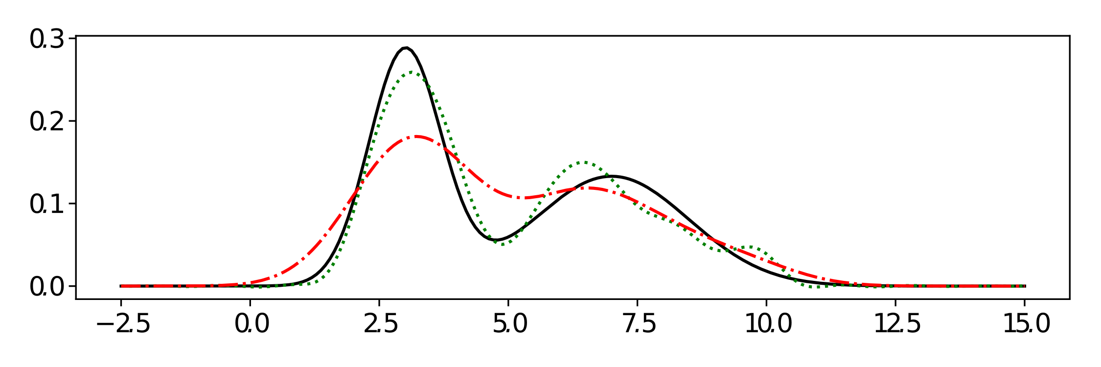
This arXival by Feng and Dicker deals with the problem of fitting multivariate mixture estimates with maximum likelihood. One of the advantages put forward being that nonparametric maximum likelihood estimators (NPMLEs) put virtually no constraints on the base measure $G_0$ . While the abstract claims their approach works for arbitrary distributions as mixture components, really they make the assumption that the components are well approximated by a Gaussian (of course including distributions arising from sums of RVs because of the CLT). While theoretically NPMLEs might put no constraints on the base measure, practically in the paper first $G_0$ is constrained to measures supported on at most as many points as there are data points. To make the optimization problem convex, the support is further constrained to a finite grid on some compact space that the data lies on.

The main result of the paper is in Proposition 1, which basically says that the finite grid constraint indeed makes the problem convex. After that the paper directly continues with empirical evaluation. I think the method proposed is not all that general. While the elliptical unimodal (gaussian approximation) assumption would not be that problematic, the claimed theoretical flexibility of NPMLE is not really bearing fruit in this approach, as the finite grid constraint is very strong and gets rid of most flexibility left after the gaussian assumption. For instance, the gaussian location model fitted is merely a very constrained KDE without even allowing the ability of general gaussian mixture models of fitting the covariance matrix of individual components. While a finite grid support for location and covariance matrix is possible, to be practical the grid would have to be extremely dense in order gain flexibility in the fit. While it is correct that the optimization problem is becoming convex, this is bought for the price of a rigid model. However, Ewan Cameron assured me that the model is very useful for astrostatistics, and I realized that it might be so in other contexts, e.g. adaptive Monte Carlo techniques.

A minor comment regarding the allegation in the paper that nonparametric models lack interpretability: while this is certainly true for the model proposed in the paper and mainstream bayesian nonparametric models, this is not a given. One notable interpretable class of models are Mixture models with a prior on the number of components by Miller and Harrison (2015).

Lifted Convex Quadratic Programming

August 17, 2016Inference, Monte Carlo, statsIngmar

This arXival by Mladenov, Kleinhans and Kersting considers taking advantage of symmetry structure in quadratic programming problems in order to speed up solvers/optimizers. The basic idea is to check which of the model parameters are indistinguishable because of symmetries in the model and assign all parameters in a group the same parameter in all steps of optimization – yielding a partition of the parameter space. Of course, this will reduce the effective dimensionality of the problem and might thus be considered a method of uncovering the lower-dimensional manifold that contains at least one optimum/solution.
The core contributions of the paper are
1) to provide the conditions under which a partition is a lifting partition, i.e. a partition such that setting all the variables in a group to the same value still includes a solution of the quadratic program
2) provide conditions under which the quadratic part of the program is fractionally symmetric , i.e. can be factorized
Furthermore, the paper touches on the fact that some kernelized learning algorithms can benefit from lifted solvers and an approximate lifting procedures when no strict lifting partition exists.

It is rather hard to read for somebody not an expert in lifted inference. While all formal criteria for presentation are fulfilled, more intuition for the subject matter could be given. The contributions of the paper are hard to grasp and more on the theoretical side (lifting partitions for convex programs can be “computed via packages such as Saucy”). While deepening the theoretical understanding a bit, it is unclear wether this paper will have a strong effect on the development of the theory of lifted inference. Even the authors seem to think that it will not have strong practical implications.

In general I wonder wether lifted inference really isn’t just an automatic way of finding simpler, equivalent models, rather than an inference technique per se.