
This is a most interesting ICML paper by Belkin, Ma and Mandal. Its starting point (as in seemingly many recent papers by Belkin) is the observation that there is robust generalisation performance of statistical models for interpolating solutions/solutions with zero training error, an observation previously made by Recht and Bengio for deep learning. The authors find that this phenomenon persists if we change the model class from deep networks to kernel machines. In particular, the non-smooth Laplacian kernel can fit random training labels in a classification problem.
On the other hand, the authors provide bounds for smooth kernels that diverge with increasing data. To arrive at this conclusion they show that the norm of interpolating solutions diverges with the number of data points (they call interpolating solutions “overfitted” which I think is not the best term). This implies divergence of generalisation bounds as well, as they depend on the norm of the solution.
The assumption needed for the theoretical results is that the label noise of the training data is nonzero. Experimentally, the paper checks how interpolating kernel classifiers perform in this case using synthetic datasets with known label noise and real world data sets with added noise. Here, the empirical test performance of the interpolating kernel classifier is slightly below the noise level, showing near optimal performance. This parallels the performance of deep networks.
The paper concludes that a deep architecture, as such, is not responsible for the good test performance of zero-training-error solutions. And as almost all bounds for RKHS methods depend on the norm of the solution, that a new theory is needed for these zero-training-error regimes. A complementary finding is that optimisation for fitting random labels is more demanding with Gaussian kernels as compared to non-smooth Laplacian kernels.
The authors conjecture that inductive bias, rather than regularisation, is particularly important in deep learning and kernel methods. Concretely, for kernel methods, the span of the canonical features at the data points 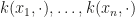
I agree with the authors in that (frequentist) kernel methods are a good place to start analysing minimum norm solutions, as here they are often available in closed form, unlike in (frequentist) deep learning.

 under the target when using Metropolis Hastings is
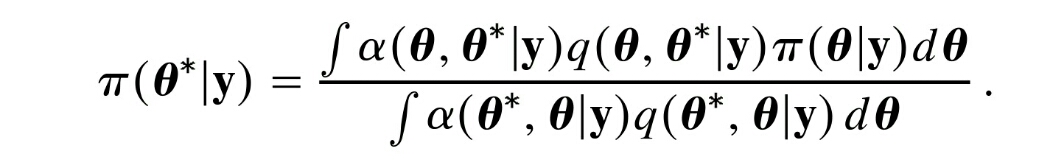
 is the proposal density,
  the acceptance probability and
  the data. If
  is the unnormalized target, we can get the evidence estimate
  .
. . The authors claim that because it is cheap to sample from
  for each sample
 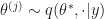 is the opposite of cheap! It involves evaluating
  for all j, which is basically the same cost as getting samples from the target in the first place.
 The basic idea is to use character level ConvNets (with a pooling operation over time), extract features using the recently proposed autobahn networks (
 some function F is submodular if
  . For a probabilistic model one can use such an F by defining a probability of a set as
 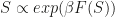 . Because of the diminishing returns, this results in a distribution where points are repulsive and tend to spread out over the space rather than clump together, just like in Low Discrepancy Point Sets used for QMC. Think Determinantal Point Process, which is log-submodular and has also been called the Antisocial Coffeshop Process, or, evocatively, the Urinal Process (thanks to Vinayak Rao for this 😀 ).
 if the base set from which we can add/remove points is of cardinality n. If adding/removing a point only has an certain effect on the submodular function bounded by 1, then the sampler mixes at least in time
  . I have no intuition wether this improved result is obtained under realistic assumptions.
 for output y, input x and parametrization of the layer given by w, a highway layer is simply given by
  , where T and C (Transfer and Carry, respectively) are functions with a (co)domain of the same dimensionality as x and y. This is called a highway layer, as gradient infomation supposedly travels faster along the $latexx \odot C(x, w_C)$ part (hence the Autobahn illustration). When it is required to change dimensionality, one has to resort to a normal layer, or subsample/pad.
 , one through
  and the output of a layer is a combination of the input of the layer x and the output of
  . The authors use a logistic model
  and
and  . The authors biased towards simply carrying information through without transformation, which in their setup means simply
  . After training the network with SGD an looking at the value of the transform gates of different layers, they find that those are closed on average (Figure 2, second column) while exhibiting large variance across inputs (exemplified by the transform gate outputs of a single sample, Figure 2, third column). Interestingly, some dimensions of the input to the network are carried through right to the last layer.
 accordingly (if it is fully connected that is). Why does adding the extra complexity gain so much? I do not feel the paper addressing this important question and I can only speculate myself: perhaps the transform/carry architecture is effective because its weights lie on a compact manifold (because of the logistic transform). Maybe the problem becomes better conditioned because simple downscaling of the input is done by T, while H takes care of actual transformations. To check this, it would have been interesting to know whether they used any constraints on the weights of H – if they haven’t, and H is fully connected, the better conditioning might be an actual explanation. In that case, simply constraining the weights
  of H (mapping input
  to the same output dimension
  ) in an appropriate way might have similar effects.