Marginal Likelihood From the Metropolis–Hastings Output

This is a rather old JASA paper by Siddhartha Chib and Ivan Jeliazkov from 2001. I dug it up again as I am frantically trying to get my contribution for the CRiSM workshop on Estimating Constants in shape. My poster will be titled Flyweight evidence estimates as it looks at methods for estimating model evidence (aka marginal likelihood, normalizing constant, free energy) that are computationally very cheap when a sample from the target/posterior distribution exists.
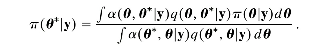
I noticed again that the approach by Chib & Jeliazkov (2001) does not satisfy this constraint, although they claim otherwise in the paper. The estimator is based on the fact that the normalized probability of a point $\theta^*$ under the target when using Metropolis Hastings is

where $q$ is the proposal density, $\alpha$ the acceptance probability and $y$ the data. If $\bar\pi$ is the unnormalized target, we can get the evidence estimate $Z = \bar\pi (\theta^*|y)/\pi(\theta^*|y)$ .
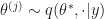
Now the integral in the numerator is cheap to estimate when we already have samples from $\pi$ . The authors claim that because it is cheap to sample from $q$ , the denominator is cheap as well. I can’t help it: this statement feels a bit deceptive to me. While indeed samples from $q$ are cheep to generate, evaluating $\alpha(\theta^*,\theta^{(j)}|y)$ for each sample $\theta^{(j)} \sim q(\theta^*,\cdot|y)$ is the opposite of cheap! It involves evaluating $\bar\pi(\theta^{(j)}|y)$ for all j, which is basically the same cost as getting samples from the target in the first place.
I already included that criticism in my PhD thesis, but when revising under time pressure I no longer thought it was valid and erroneously took it out.