Category Archives: Inference

Overdispersed Black-Box Variational Inference

June 22, 2016Inference, Monte Carlo, stats, Variational InferenceIngmar

This UAI paper by Ruiz, Titsias and Blei presents important insights for the idea of a black box procedure for VI (which I discussed here). The setup of BBVI is the following: given a target/posterior $\pi$ and a parametric approximation $q_\lambda$ , we want to find

$\mathrm{argmin}_\lambda \int \log \left ( \frac{\pi(x)}{q_\lambda(x)} \right ) q_\lambda(x) \mathrm{d}x$

which can be achieved for any $q_\lambda$ by estimating the gradient

$\nabla_\lambda \int \log \left ( \frac{\pi(x)}{q_\lambda(x)} \right ) q_\lambda(x) \mathrm{d}x$

with Monte Carlo Samples and stochastic gradient descent. This works if we can easily sample from $q_\lambda$ and can compute its derivative wrt $\lambda$ in closed form. In the original paper, the authors suggested the use of the score function as a control variate and a Rao-Blackwellization. Both where described in a way that utterly confused me – until now, because Ruiz, Titsias and Blei manage to describe the concrete application of both control variates and Rao-Blackwellization in a very transparent way. Their own contribution to variance reduction (minus some tricks they applied) is based on the fact that the optimal sampling distribution for estimating $\nabla_\lambda \int \log \left ( \frac{\pi(x)}{q_\lambda(x)} \right ) q_\lambda(x) \mathrm{d}x$ is proportional to $\left | \log \left ( \frac{\pi(x)}{q_\lambda(x)} \right ) \right | q_\lambda(x)$ rather than exactly $q_\lambda(x)$ . They argue that this optimal sampling distribution is considerably heavier tailed than $q_\lambda(x)$ . Their reasoning is mainly that the norm of the gradient (which is essentially $(\nabla_\lambda q_\lambda) \log \left ( \frac{\pi(x)}{q_\lambda(x)} \right ) = q_\lambda(x)(\nabla_\lambda \log q_\lambda(x)) \log \left ( \frac{\pi(x)}{q_\lambda(x)} \right )$ ) vanishes for the modes, making that region irrelevant for gradient estimation. The same should be true for the tails of the distribution I think. Overall very interesting work that I strongly recommend reading, if only to understand the original Blackbox VI proposal.

A Variational Analysis of Stochastic Gradient Algorithms

May 9, 2016big tall data, Inference, mcmc, Monte Carlo, stats, tall big data, Variational InferenceIngmar

This arXival by Mandt, Hoffman and Blei from February takes a look at what they call SGD with constant learning rate or constant SGD. Which is not really Stochastic Gradient Descent anymore, but rather a sampling algorithm, as we should bounce around the mode of the posterior rather than converging to it. Consequently they interpret constant SGD as a stochastic process in discrete time with some stationary distribution. They go on to analyse it under the assumption that the stationary distribution is Gaussian (Assumption 1 and 4). Something that springs to my mind here is the following: even if we accept that the stationary distribution of the process might be Gaussian (intuitively, not rigorously), what guarantees that the stationary distribution is the posterior? Even if the posterior is also gaussian, it could have a different (co)variance. I think a few more words about this question might be good. In particular, without adding artificial noise, is it guaranteed that every point in the posteriors domain can be reached with non-zero probability? And can be reached an infinite number of times if we collect infinite samples? If not, the constant SGD process is transient and does not enjoy good stability properties.

Another delicate point hides in Assumption 1: As our stochastic gradient is the sum of independent RVs, the CLT is invoked to assume that the gradient noise is Gaussian. But the CLT might not yet take effect if the number of data points in our subsample is small, which is the very thing one would like in order to have advantages in computation time. This of course is yet another instance of the dilemma common to all scalable sampling techniques, and at this stage of research this is not a show stopper.
Now assuming that constant SGD is not transient and it has a stationary distribution that is the posterior and that the posterior or its dominant mode is approximately Gaussian, we can of course try to optimize the parameters of constant SGD to make the sample it produces as close a possible to a posterior sample. Which the authors conveniently do using an Ornstein-Uhlenbeck approximation, which has a Gaussian stationary distribution. Their approach is to minimize KL-Divergence between the OU approximation and the posterior, and derive optimal parameter settings for constant SGD in closed form. The most interesting part of the theoretical results section probably is the one on optimal preconditioning in Stochastic Gradient Fisher Scoring, as that sampler adds artificial noise. Which might solve some of the transience questions.

The presentation would gain a lot by renaming “constant SGD” for what it is – a sampling algorithm. The terminology and notation in general are sometimes a bit confusing, but nothing a revision can’t fix. In general, the paper presents an interesting approach to deriving optimal parameters for a class of algorithms that is notoriously hard to tune. This is particularly relevant because the constant step size could improve mixing considerably over Welling & Tehs SGLD. What would be interesting to see is wether the results could be generalized to the case where the posterior is not Gaussian. For practical reasons, because stochastic VB/EP works quite well in the gaussian case. For theoretical reasons, because EP now even comes with some guarantees (haven’t read that paper admittedly). Maybe a path would be to take a look at the Gaussian approximation to a multimodal posterior spanning all modes, and minimizing KL-Divergence between that and the OU process. Or maybe one can proof that constant SGD (with artificial noise?) has some fixed stationary distribution to which stochastic drift term plus noise are a Markov Kernel, which might enable a pseudo-marginal correction.

Variational Hamiltonian Monte Carlo via Score Matching

April 26, 2016Inference, mcmc, Monte Carlo, Neural Networks, stats, Variational InferenceIngmar

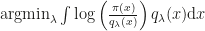
This is an arXival (maybe by now ICML paper?) by Zhang, Shahbaba and Zhao. It suggest fitting an emulator/surrogate $q_\eta$ to the target density $\pi$ via score matching and then use the gradients of $q_\eta$ rather than those of $\pi$ for generating proposal with HMC. Their main selling point being that this decreases wall-clock time for HMC.

However, that seems to me like reselling the earlier paper by Heiko Strathmann and collaborators on Gradient-free Hamiltonian Monte Carlo with Efficient Kernel Exponential Families. Zhang et al use basically the same idea but fail to look at this earlier work. Their reasoning to use a neural network rather than a GP emulator (computation time) is a bit arbitrary. If you go for a less rich function class (neural network) then the computation time will go down of course – but you would get the same effect by using GPs with inducing points.

Very much lacking to my taste is reasoning for doing the tuning they do. Sometimes they tune HMC/Variational HMC to 85% acceptance, sometimes to 70% acceptance. Also, it seems they not adapting the mass matrix of HMC. If they would, I conjecture the relative efficiency of Standard HMC vs Variational HMC could change drastically. Details on how they tune SGLD is completely lacking.

Overall, I think it is not yet clear what can be learned from the work reported in the paper.

Non-asymptotic convergence analysis for the Unadjusted Langevin Algorithm

April 15, 2016Inference, mcmc, Monte Carlo, Numerics, statsIngmar

This is an important arXival by Alain Durmus and Eric Moulines. The title is slightly optimized for effect, as the paper actually contains non-asymptotic and asymptotic analysis.

The basic theme of the paper is in getting upper bounds on total variation (and more general distribution distances) between an uncorrected discretized Langevin diffusion wrt some target $\pi$ and $\pi$ itself. The discretization used is the common scheme with the scary name Euler-Maruyama:

$X_{k} \sim \mathcal{N}(\cdot|X_{k-1} + \gamma_{k}\nabla \log \pi(X_{k-1}), \sqrt{2\gamma_{k}I} = R_{\gamma_{k}}(\cdot |X_{k-1})$

Under a Foster-Lyapunov condition, $R_{\gamma_{k}}$ is a Markov kernel that admits a unique stationary distribution $\pi_{\gamma_{k}}$ that is close to the desired $\pi$ in total variation distance and gets closer when $\gamma_{k}$ decreases.

Now in the non-asymptotic case with fixed $\gamma = \gamma_k$ , the authors provide bounds that explicitly depend on dimensionality of the support of the target, the number of samples drawn and the chosen step size $\gamma$ . Unfortunately, these bounds contain some unknowns as well, such as the Lipschitz constant $L$ of the gradient of the logpdf $\log \pi(\cdot)$ and some suprema that I am unsure how to get explicitly.

Durmus and Moulines particularly take a look at scaling with dimension under increasingly strong conditions on $\pi$ , getting exponential (in dimension) constants for the convergence when $\pi$ is superexponential outside a ball. Better convergence can be achieved when assuming $\pi$ to be log-concave or strongly log-concave. This is not surprising, nevertheless the theoretical importance of the results is clear from the fact that together with Arnak Dalalyan this is the first time that results are given for the ULA after the Roberts & Tweedie papers from 1996.

As a practitioner, I would have wished for very explicit guidance in picking $\gamma$ or the series $\{\gamma_k\}_{k=1}^\infty$ . But hopefully with Alains paper as a foundation that can be the next step. As a non-mathematician, I had some problems in following the paper and at some point I completely lost it. This surely is in part due to the quite involved content. However, one might still manage to give intuition even in this case, as Sam Livingstones recent paper on HMC shows. I hope Alain goes over it again with readability and presentation in mind so that it will get the attention it deserves. Yet another task for something that already took a lot of work…

(photo: the Lipschitz Grill diner in Berlin – I don’t
know about their food, but the name is remarkable)

Quasi-Monte Carlo Methods in Finance

March 9, 2016Inference, Monte Carlo, Numerics, Quasi Monte CarloIngmar

This second reference Mathieu Gerber gave me in the quest for educating myself about QMC, is paper by Pierre L’Ecuyer from the Winter Simulation Conference in 2004. It was much clearer as a tutorial (for me) as compared to the Art Owen paper. Maybe because it didn’t contain so much ANOVA. Or maybe because I was more used to ANOVA from Arts paper.

This paper specifically and quite transparently treats different constructions for low discrepancy point sets, in particular digital nets and their special cases. On the other hand, randomization procedures are discussed, which sometimes seem to be very specialized to the sequence used. One seemingly general transform after randomization called the baker transformation results in surprisingly high variance reduction of order $O(n^{-4+\epsilon})$ . The transformation being to replace the uniform coordinate $u \in [0,1)$ by $2u$ for $u\leq 0.5$ and $2(1-u)$ else.

In the examples L’Ecuyer mentions that using an Eigenzerlegung of covariance matrices (i.e. PCA) results in much higher variance reductions as compared to using Cholesky factors. Which he attributes to dimension reduction – a naming I find odd, as the complete information is retained (as opposed to, e.g. tossing the components with lowest Eigenvalue). My intuition is that maybe the strong empirical gains with PCA might rather be attributed to the fact that Eigenvectors are orthogonal, making this decomposition as close as possible to QMCs beloved unit hypercube.

Monte Carlo Extension of Quasi-Monte Carlo

March 7, 2016Inference, Monte Carlo, NumericsIngmar

405px-Subrandom_2D — Low discrepancy (top) vs. randomly uniform points (bottom)

Mathieu Gerber gave me this 1998 paper by Art Owen as one of several references for good introductions to QMC in the course of evaluating an idea we had at MCMSki.

The paper surveys re-randomization of low discrepancy/QMC point sets mostly as a way of getting an estimate of the variance of the integral estimate. Or that is what the paper makes states most prominently – another reason for doing randomized QMC being that in some cases it further decreases variance as compared to plain QMC.

One of the things this paper stresses is that QMC will not help in truly high-dimensional integrands: say you have a $d$ dimensional integrand which does not live on a lower dimensional manifold, and only use $n \ll O(d^2)$ . Then equidistributing these $n$ points meaningfully in becomes impossible. Of course if the integrand does live on a lower dimensional manifold, one can use that fact to get convergence rates that correspond to the dimensionality of that manifold, which corresponds (informally) to what Art Owen calls effective dimension. Two definitions of effective dimension variants are given, both using the ANOVA decomposition. ANOVA only crossed my way earlier through my wifes psychology courses in stats, where it seemed to be a test mostly, so I’ll have delve more deeply into the decomposition method. It seems that basically, the value of the integrand $f(x_1,\dots,x_d)$ is treated as a dependent variable while the $x_1, \dots, x_d$ are the independent variables and ANOVA is used to get an idea of how independent variables interact in producing the dependent variable. In which case of course we would have to get some meaningful samples of points $(x_1,\dots,x_d, f(x_1,\dots,x_d))$ which currently seems to me like circling back to the beginning, since meaningful samples are what we want in the first place.

The idea for getting variance of the integral estimate from RQMC is the following: given a number $m$ of deterministic QMC points, randomize them $r$ times using independently drawn random variables. The integral estimates $\hat I_1,\dots, \hat I_r$ are unbiased estimates of the true integral $I$ with some variance $\sigma_{\textrm{RQMC}}^2$ . Averaging over the $latex \hat I_i$ we get another unbiased estimator $latex \hat I$ which has variance $\sigma_{\textrm{RQMC}}^2/r$ . This RQMC variance can be estimated unbiasedly as $\frac{1}{r(r-1)} \sum_{i=1}^r (\hat I_i - \hat I)^2$ . If $m = 1$ then $r$ is the number of samples and this simply is the standard estimate of Monte Carlo variance.

The paper goes on to talk about using what it calls Latin Supercube Sampling for using RQMC in even higher dimensions, again using ANOVA decomposition and RQMC points in each group of interacting variables as determined by the ANOVA.

Overall, I know a bit more about QMC but am still more in the confusion than the knowledge state, which I hope Mathieus next reference will help with.

Kernel Sequential Monte Carlo

February 15, 2016Importance Sampling, Inference, Monte Carlo, SMCIngmar

Heiko Strathmann, Brooks Paige, Dino Sejdinovic and I updated our draft on Kernel Sequential Monte Carlo (on the arxiv). Apart from locally adaptive covariance matrices for Gaussian proposals in various SMC algorithms, we also look at gradient emulators – both for targets that do not admit a first (gradient emulators) or even second derivative (locally adaptive covariance).
The emulators can be used in different ways, either as proposals for a MCMC rejuvenation step in SMC or as importance densities directly – for example in Population Monte Carlo.
We found especially the gradient emulator to be rather sensitive to the variance of the fit. Not Rao-Blackwellizing across importance densities used in a PMC iteration leads to gigantic estimated gradients and an exploding algorithm, while using a weighted streaming fit of the emulator with Rao-Blackwellization works just fine.
Plus we evaluate on the Stochastic volatility target from Nicolas SMC^2 paper, which is a much more nicer benchmark that what we had in the last draft (the plot being the targets marginals). Any feedback please send my way.

On the Geometric Ergodicity of Hamiltonian Monte Carlo

February 10, 2016Inference, mcmc, Monte Carlo, Numerics, statsIngmar

This remarkable arXival by Sam Livingstone, Betancourt, Byrne and Girolami takes a look at the conditions under which Hybrid/Hamiltonian Monte Carlo is ergodic wrt a certain distribution $\pi$ , and, in a second step, under which it will converge in total variation at a geometric rate. A nice feature being that they even prove that setting the integration time dynamically can lead to the sampler yielding geometric rate for a larger class of targets. Under idealized conditions for the dynamic integration time and, admittedly, in a certain exponential family.

Whats great about this paper, apart from the results, is how it manages to give the arguments in a rather accessible manner. Considering the depth of the results that is. The ideas are that

the gradient should at most grow linearly
for the gradient of $\pi$ to be of any help, it cannot lead further into the tails of the distribution or vanish (both assumption 4.4.1)
as we approach infinity, every proposed point thats closer to the origin will be accepted (assumption 4.4.2)

If the gradient grows faster than linear, numerics will punch you in the face. That happened to Heiko Strathmann and me just 5 days ago in a GradientIS-type algorithm, where an estimated gradient had length $10^{144}$ and led to Nirvana. If not the estimation is the problem but the actual gradient, of course you have the same effect. The second assumption is also very intuitive: if the gradient leads into the tails, then it hurts rather than helps convergence. And your posterior is improper. The final assumption basically requires that your chance to improve by proposing a point closer to the origin goes to $1$ the further you move away from it.

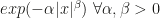
A helpful guidance they provide is the following. For a class of exponential family distributions given by $exp(-\alpha|x|^\beta)~\forall \alpha,\beta >0$ , whenever the tails of the distribution are no heavier than Laplace ( $\beta \geq 1$ ) and no thinner than Gaussian ( $\beta \leq 2$ ), HMC will be geometrically ergodic. In all other cases, it won’t.

Another thing that caught my eye was their closed form expression for the proposal after $L$ leapfrog steps with stepsize $\epsilon$ , eq. (13):

Capture d’écran 2016-02-09 à 21.28.00

Which gives me hope that one should be able to compute the proposal probability after any number of leapfrog steps as long as $\nabla \log \pi$ is invertible and thus a Jacobian exists to account for the transformation of $p_0$ hidden in the $x_{i\epsilon}$ . A quick check with $\pi$ given by a bayesian posterior shows that this might not be trivial however.

A Repulsive-Attractive Metropolis Algorithm for Multimodality

January 26, 2016Inference, mcmc, Monte CarloIngmar

(Title image from Wikipedia)

Christian put my nose on this preprint by Tak, Meng and van Dyk a few days ago, so during the flight from Berlin to Paris today I sniffed on it. It was a very interesting read and good to get my thoughts away from the fact that I was an Opfer of German friendliness at airport security.
The basic idea is to design a random walk MH algorithm for targets with multiple and distant modes. The distant is important here, because for very close modes simple Adaptive Metropolis (Haario et al. 2001), which is simply using a scaled version of the targets covariance in a Gaussian random walk, should work pretty well.

Which it probably does not for the targets above, as such a proposal would often end up in areas of low posterior density.
Now the idea is the following: given current state $x_i$ of the Markov Chain, the final MH proposal $x''$ is constructed using an intermediate step $x'$ , where the intermediate step is encouraged to have lower density than $x_i$ under the target, while $x''$ is encouraged to have higher density than the intermediate step. Hoping that the intermediate step gets you out of a mode and the consecutive step into a new mode. This is achieved by using the inverse MH-ratio for encouraging moves to a valley in the target, while the standard MH-ratio is used for moving uphill again. Of course computing the final acceptance probability $\alpha(x''|x_i)$ involves computing an intractable integral, as one has to integrate away the intermediate downhill move. They get around this by introducing an auxiliary variable, a technique inspired by Møller et al. (2006), where it was used to get around the computation of normalizing constants. I discussed a similar idea shortly with Jeff Miller (currently at Duke) one and a half years ago when we worked on the estimation of normalizing constants though using gradient information.
Am main argument for their algorithm is that it only needs tuning of a single scale parameter, whereas other MCMC techniques for multimodal targets are notoriously hard to tune.
In evaluation they compare to tempered transitions and equi-energy samplers and perform better both with respect to computing time and MSE. And of course human time invested in tuning.
However, I’m slightly tempted to repeat Nicolas mantra here “just use SMC”. Or slightly change the mantra to “… PMC” – because this is easier to stomach for MCMC-biased researchers, or so I believe. Of course this adds the number of particles to tuning, but that might be tuned automatically using the recent paper of the Spanish IS-connection.

Layered adaptive Importance Sampling

January 25, 2016Inference, mcmc, SMCIngmar

This arXival from last spring/summer by Martino, Elvira, Luengo and Corander combines and extends upon recent advances of Importance Sampling, using mainly ideas from Adaptive Multiple lmportance Sampling (AMIS) and Population Monte Carlo (PMC). The extension consists of the idea to not use the Importance Sampling procedure itself to come up with new proposal distributions, but rather to run a Markov Chain. The output of which is used solely as the location parameter for IS proposal distributions $q_{n,t}$ . The weights of the samples drawn from these are Rao-Blackwellized using the deterministic mixture idea of Zhou and Owen, and as far as I can see only the Importance Samples are used for estimating integrands.
What’s most striking for me as somebody who has thought about these methods a lot during the PhD is the idea that in principle one is free to Rao-Blackwellize using an arbitrary partition of the samples/proposal distributions and still get a consistent estimator. Xi’an mentioned this to me earlier and of course it is not surprising given that even without Rao-Blackwell my Gradient IS did considerably better than some Adaptive MCMC algorithms. However this paper makes that idea transparent and uses it extensively. The main idea that is put forward however is to use (parallel) MCMC with the same target for coming up with IS-proposal locations. The output of MCMC is only used for that purpose but not for estimation. Which seems kind of wasteful, but in a nice conversation over email the first author Luca Martino assured me that recycling proposals as both IS and MH proposals made performance go down because of correlations. I don’t get an intuition for why that would be the case, but maybe I’ll have to fall on my own nose for that. What I like about this particular idea of getting locations from MCMC is that one is free from the tuning problem I’ve hit upon in GRIS: if you scale up the proposal covariance in GRIS (or in the PMC approach from the Cappé 2004 paper), you can get an arbitrarily high ESJD – together with a really bad target approximation. Thus unmodified ESJD cannot be used for tuning. And neither can acceptance rate which doesn’t exist. Using MCMC for getting proposal locations is an elegant way around that problem. The effect of this is shown in the plot from the paper below, where the two rightmost plots show one of their methods.

Some other aspects about the paper I find less clear. For instance, I’m not sure about the abundance of different algorithms that are introduced. It leaves the impression that the authors where trying to do mass instead of class (something I might make myself guilty of these weeks as well). Also, while the targets they use for evaluation are fine, only reporting the MSE of one dimension of one integrand seems odd. One simple thing here might be to report the MSE averaged over dimensions as well, another to report the MSE of an estimate of the target distributions variance/higher order moments.

(Title image (c) Carlos Delgado, CC-BY-SA)