On behalf of the mcqmc 2016 organizing committee I am pleased to accept your proposal.
-Art Owen
I got this nice message from Art yesterday night. My proposal for a session on
Advances in Importance Sampling at
MCQMC 2016 got accepted. Which is great, as I think the session is made up of strong papers (obviously). This session will almost surely be moderated by
Nicolas Chopin.
MCQMC session on Advances in Importance Sampling
The sample size required in Importance Sampling
S. Chatterjee, P. Diaconis
The goal of importance sampling is to estimate the expected value of a given function with respect to a probability measure ν using a random sample of size n drawn from a different probability measure μ. If the two measures μ and ν are nearly singular with respect to each other, which is often the case in practice, the sample size required for accurate estimation is large. In this article it is shown that in a fairly general setting, a sample of size approximately exp(D(ν||μ)) is necessary and sufficient for accurate estimation by importance sampling, where D(ν||μ) is the Kullback–Leibler divergence of μ from ν. In particular, the required sample size exhibits a kind of cut-off in the logarithmic scale. The theory is applied to obtain a fairly general formula for the sample size required in importance sampling for exponential families (Gibbs measures). We also show that the standard variance-based diagnostic for convergence of importance sampling is fundamentally problematic. An alternative diagnostic that provably works in certain situations is suggested.
Generalized Multiple Importance Sampling
V. Elvira, L. Martino, D. Luengo, M. Bugallo
Importance Sampling methods are broadly used to approximate posterior distributions or some of their moments. In its standard approach, samples are drawn from a single proposal distribution and weighted properly. However, since the performance depends on the mismatch between the targeted and the proposal distributions, several proposal densities are often employed for the generation of samples. Under this Multiple Importance Sampling (MIS) scenario, many works have addressed the selection or adaptation of the proposal distributions, interpreting the sampling and the weighting steps in different ways. In this paper, we establish a general framework for sampling and weighing procedures when more than one proposal are available. The most relevant MIS schemes in the literature are encompassed within the new framework, and, moreover novel valid schemes appear naturally. All the MIS schemes are compared and ranked in terms of the variance of the associated estimators. Finally, we provide illustrative examples which reveal that, even with a good choice of the proposal densities, a careful interpretation of the sampling and weighting procedures can make a significant difference in the performance of the method.
Continuous-Time Importance Sampling
K. Łatuszyński, G. Roberts, G. Sermaidis, P. Fearnhead
We will introduce a new framework for sequential Monte Carlo, based on evolving a set of weighted particles in continuous time. This framework can lead to novel versions of existing algorithms, such as Annealed Importance Sampling and the Exact Algorithm for diffusions, and can be used as an alternative to MALA for sampling from a target distribution of interest. These methods are amenable to the use of sub-sampling, which can greatly increase their computational efficiency for big-data applications; and can enable unbiased sampling from a much wider-range of target distributions than existing approaches.


 under the target when using Metropolis Hastings is
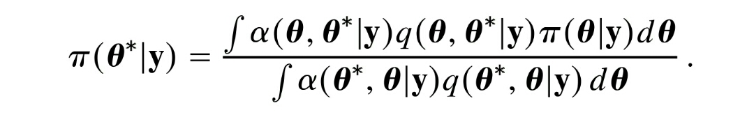
 is the proposal density,
  the acceptance probability and
  the data. If
  is the unnormalized target, we can get the evidence estimate
  .
. . The authors claim that because it is cheap to sample from
  for each sample
  is the opposite of cheap! It involves evaluating
  for all j, which is basically the same cost as getting samples from the target in the first place.

 is a Markov kernel that admits a unique stationary distribution
  that is close to the desired
  decreases.
 , the authors provide bounds that explicitly depend on dimensionality of the support of the target, the number of samples drawn and the chosen step size
  . Unfortunately, these bounds contain some unknowns as well, such as the Lipschitz constant
  of the gradient of the logpdf
  and some suprema that I am unsure how to get explicitly.
 . But hopefully with Alains paper as a foundation that can be the next step. As a non-mathematician, I had some problems in following the paper and at some point I completely lost it. This surely is in part due to the quite involved content. However, one might still manage to give intuition even in this case, as Sam Livingstones recent


 . The transformation being to replace the uniform coordinate
  by
by  for
for  and
and  else.
else.
 dimensional integrand which does not live on a lower dimensional manifold, and only use
  . Then equidistributing these
  points meaningfully in becomes impossible. Of course if the integrand does live on a lower dimensional manifold, one can use that fact to get convergence rates that correspond to the dimensionality of that manifold, which corresponds (informally) to what Art Owen calls effective dimension. Two definitions of effective dimension variants are given, both using the ANOVA decomposition. ANOVA only crossed my way earlier through my wifes psychology courses in stats, where it seemed to be a test mostly, so I’ll have delve more deeply into the decomposition method. It seems that basically, the value of the integrand
  is treated as a dependent variable while the
  are the independent variables and ANOVA is used to get an idea of how independent variables interact in producing the dependent variable. In which case of course we would have to get some meaningful samples of points
  which currently seems to me like circling back to the beginning, since meaningful samples are what we want in the first place.
 of deterministic QMC points, randomize them
  times using independently drawn random variables. The integral estimates
  are unbiased estimates of the true integral
  with some variance
  . Averaging over the $latex \hat I_i$ we get another unbiased estimator $latex \hat I$ which has variance
  . This RQMC variance can be estimated unbiasedly as
  . If
. If  then
then 

